An attempt to extend xG gain
Some time ago I was reflecting on a good way of valuing passes and came across this idea: we can treat the situations right before and right after a pass as goal scoring opportunity, assign xG[1] value to those situation and measure gain in xG that this pass generated. However, I got the feeling from the very beginning that this certainly cannot be new. ‘As the concept is really simple, it must have been already invented by someone’ - I thought. And indeed, valuing passes this way has already been discussed here and here. However, high xG values are obviously limited to the area close to the goal, so all passes targeted deeper on the pitch cannot be adequately rewarded, as a difference in their starting and ending xG values is usually very tiny. That makes a lot of great passes insignificant in comparison with most of passes made into penalty area. Therefore, I have made an attempt to approach this main limitation in my analysis.
The data used in this analysis contained all games from English Premier League 2017/2018. Particularly, the xG model was build based on 9218 shots and it may be the source of uncertainty. Due to scarce sample size, I resigned from traditional training/test set split and decided to employ all observations using stratified cross-validation which should give us a nice estimate of true error. Besides, as I wanted a model that extrapolates well from typical shots locations to all passes locations, logistic regression seemed to be the best choice. Finally, the model was intended to calculate xG situations before and after the pass, so I needed general features that could be used to characterise both shot and pass events. Selected features were:
distance- distance from the middle of a goalangle- angle between a goal line and a line connecting shot location and middle of a goalgame_state- in-game goal differenceseq_direct_speed- difference in x coordinate between last and first action in the sequence, divided by the total time of the sequence[2]assisted- whether a shot was assisted or not
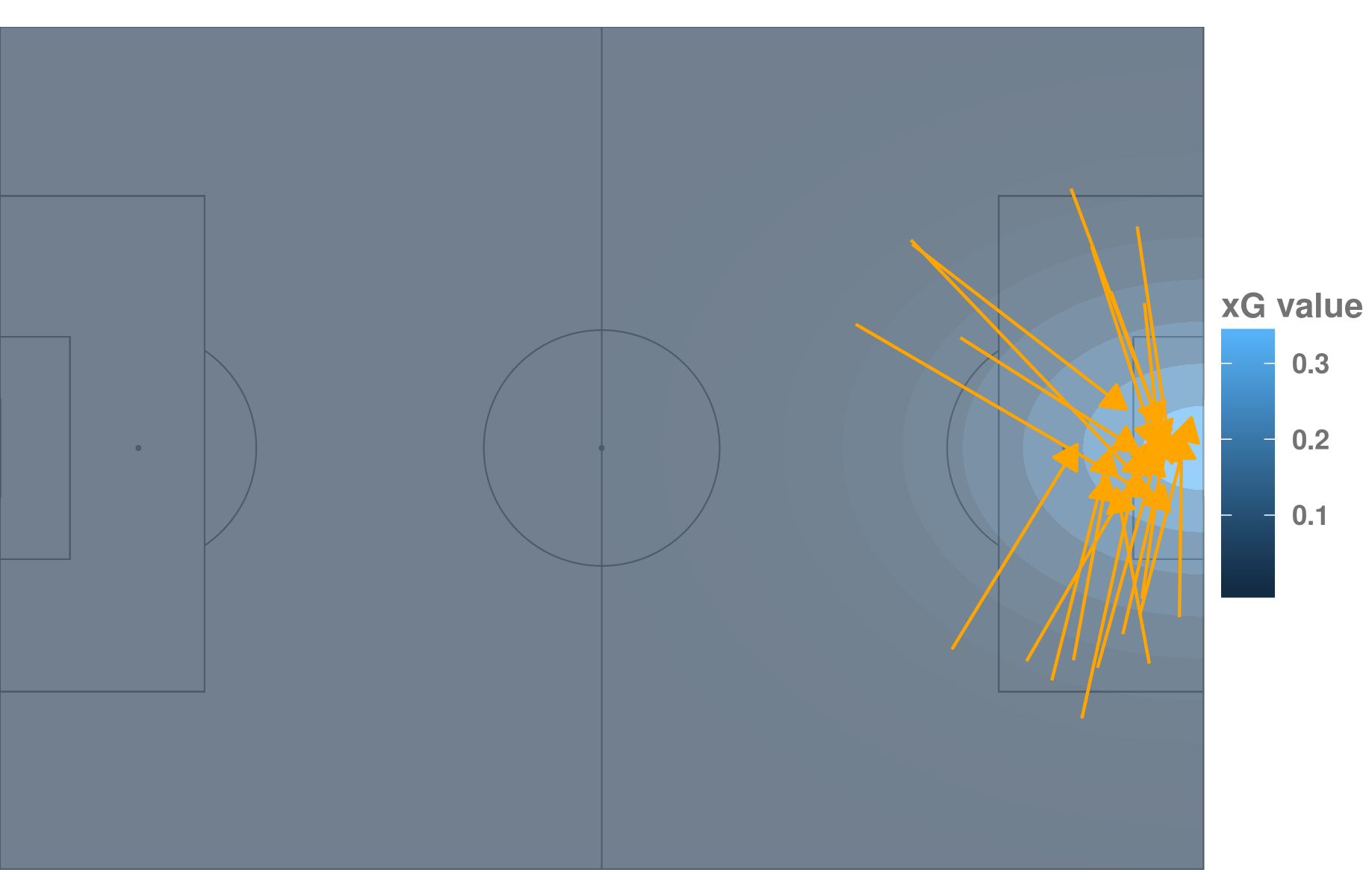
In particular, xG is a function of distance from the middle of a goal. What’s more this distance has by far the major effect in our model.[3] From the perspective of passes targeted deeper in the pitch that is a huge limitation. The graphic below shows averaged within zones xG values as well as top twenty passes with respect to xG gain and should help to see this issue. We can observe that all passes with high xG gain starts in the zones with low xG (all <0.10, coloured with different hues of dark blue, dependently on the aggerated value of xG in particular zone) and ends in the two zones with highest xG values (>0.22, coloured with light green or yellow). These few zones between forms a band. Crossing this band with a pass produces the highest xG gain (thus I will refer to it as highest-xG-gain band). It’s also clear that high xG gain values are dominated with passes targeted towards the area close to the goal. So I looked for a transformation that would partly offset marginal effect of distance from our model and move the highest-xG-gain band away from the goal. That would allow us to boost the reward for passes made deeper in the pitch, while still taking into account crucial passes made into the area close to the goal.
Technicalities
(If you’re not interested in technical stuff, you can easily skip to the Applications)
For a moment, let’s forgive that our model has features other than distance. In this setting we can assume that xG values are of the following form:
\[\begin{align*} f(x) = \exp(-(d(x, x_0))^\frac{1}{a}), \end{align*}\]where \( d(x, x_0) \) is a distance between shot location \(x\) and center of a goal \(x_0\). For \(a = 1/2\) this would be a density of bivariate normal distribution (up to the constant). On the other hand:
\[\begin{align*} f(x) = g(d(x, x_0)), \end{align*}\]where \(g\) can be identified with xG model. Therefore, to offset the marginal effect of distance we can inverse \(g\) and apply \(g^{-1}\) to xG values. The inverse function is:
\[\begin{align*} g^{-1}(f(x)) = \left(\ln\frac{1}{f(x)}\right)^a. \end{align*}\]Since it requires \(f(x) > 0\), we introduce technical shift parameter \(s\) and end up with the family of transformations \(F\) defined as:
\[\begin{align*} F(f)(x) = \left( \ln \frac{1+s}{f(x) + s} \right) ^ a. \end{align*}\]Lastly, as the xG values after transformation should lie in \([0, 1]\) as well, we normalise \(F\) obtaining:
\[\begin{align*} F(f)(x) = \left( \frac{\ln{\frac{1+s}{f(x)+s}}}{\ln{\frac{1+s}{s}}} \right) ^ a. \end{align*}\]Application
Having xG model, one can assign gain in xG values that each pass generates. To reward passes targeted deeper than the light area I will need a transformation that boosts lower and stagnate higher xG values, while still maps onto \([0,1]\). In mathematical jargon that would mean I will need a concave, bijective transformation. Although \(1 - F\) is not concave in general, I can pick the \(a, s\) parameters so that it is satisfied. It’s hard to assign the intuition for a and s separately, but generally, both parameters together control how much farther away from a goal we push this highest-xG-gain band and therefore, where we reward passes the most. Parameter a is sufficient to do this up to a certain point, s is kind of a helper here to push the highest-xG-gain band even deeper in the pitch. To see how those parameters affect the form of \(F\), please visit this basic ShinyApp I have prepared. By sliding the bars in the left upper corner you can observe how \(1 - F\) changes (right below the bars) and how it affect xG values (on the right). In fact, keeping \(s\) to default value and varying \(a\) suffices to vary from identity to the function so concave, that it is almost tangential to the point \((0, 1)\).[4]
For the purpose of this post, I will consider three forms of \(F\). Keeping \(s\) parameter constant, I will set \(a\) to 32, 256 and 2048. These values were selected because they are equidistant on logarithmic scale and approximetely refer to height of three prominent zone in the context of advancing the ball - penalty area, final third and offensive half. But let’s start with raw xG gain values. Results are limited to players who played at least 1000 minutes during Premier League 2017-2018 season.
Please note that due to the transformation form, xG gain values are not comparable accross different parameters’ values.
![]()
The results generally meet our expectations. The top 20 consists mostly with offensive players or highly attacking inclined full backs, like Trippier, Bellerin, Walker or Azpillicueta. Except for Mahrez, all players are from top-six teams. From the less obvious names we have Anthony Martial and Alex Iwobi - both seem to generate much offensive value despite the fact that they didn’t always made the starting line up. And at the top of list there are three great playmakers - Oezil, Coutinho and De Bruyne.
Penalty Area
![]()
With the first considered transformation we can observe some rotation at the top, suggesting that Fabregas probably provided some succesful passes into penalty area, but not targeted that close to the goal. There’s also an increased number of defenders among the top 20, with Kieran Trippier right outside the top 3. One interesting name here is Jonjo Shelvey, who gets even higher in the list when we consider both succesful and unsuccesful passes. This suggests that he provides a decent number of passes targeted into penalty area, but it comes at a price of many failed attempts. Other interesting names at the tail of top-20 list are Mousa Dembele, Danilo and Chris Brunt.
Final third
As this transformation offsets the distance effect pretty deep in the pitch, the list of top 20 have been dominated by defenders, who usually operate, and therefore start their passes much deeper. For this reason I present two top 10 lists - for defenders and midfielders separately.
![]()
The names of defenders are consistent with the former transformation. Among midfielders, Young and Delph - who usually played as full backs - show up at the top. Fabregas and Shelvey are still among the top, followed by Brunt and Dembele, who got slightly ahead of Oezil. This may suggest the large parts of their gains are just passes targeted into deeper regions of final third, making them potentially useful at breaking the lines.
Offensive half
![]()
With this transformation, finally some centre backs are getting rewarded enough. The presence of City defenders - Kompany and Stones - as well as two Spaniards - Monreal and Azpillicueta - is obviously expectable. Spurs’ summer signing Davinson Sanchez seem to be quite good at building out of the back too. Excluding from midfielders all players who usually played as full backs, we are left with names like Marc Albrighton, Declan Rice, Ryan Fraser and again - Cesc Fabregas, Chris Brunt and Jonjo Shelvey.
Conclusions
Choosing different forms of \(1 - F\) transformation could be potentially a powerful tool to move the highest-xG-gain bands away from the goal and bring out great passes made deeper in the pitch. Although the analysis rely on subjective, rough choices of the exact form of \(1 - F\), the results seem to pass the eye test, while still reveal some few interesting names. It has to be noted that:
- while analysing the results we have to allow for team’s playing style as it may affect the transformed xG gain scores
- the family of transformations that has been proposed is not stated to be the best - there is a bunch of mathematical functions that would do the job as well and I encourage you to take the code and experiment with different transformations.[5]
To play yourself with different functions from the defined family and look how the top 20 list is changing accross them, please go to the ShinyApp. Those who have access to OptaPro data are also encouraged to check out the code stored here.
Any feedback is highly appreciated - my e-mail address and twitter account are visible at the bottom of the page.
Acknowledgments: This work has been done as part of NYA Fellowship sponsored by North Yard Analytics. The data was provided as a courtesy of OptaPro.
[1] Expected Goals, read more on the concept here.
[2] Sequences are defined as fragments of plays that belongs to one team and are ended by any shot, defensive action, own error or stoppage in play. They are aimed to be consistent with OptaPro definition, although some minor differences can occur.
[3] According to standardised coefficients.
[4] In fact, due to the complicated form of \(1 - F\) and its dependence on xG values, it’s not possible to calculate \(a\) and \(s\) values that would make \(1 - F\) an identity function in general case. Therefore, the default values \(a = 1\) and \(s=3276.8\) don’t make \(1 - F\) an identity function exactly, but the difference seems to be negligible.
[5] The other, much simpler family of transformations that I considered was \(G(d) = \frac{d}{d+a}\). Nonetheless, the transformation presented in Technicalities section has been superior in my eyes due to its relationship with bivariate normal distribution.